Three isotopes of carbon are found in nature; carbon-12, carbon-13 and carbon-14.   Carbon-12 accounts for ~99.8 % of all carbon atoms, carbon-13 accounts for ~1% of carbon atoms while ~1 in every 1 billion carbon atoms is carbon-14.  Hereafter these isotopes will be referred to as 12C, 13C, and 14C.  14C is radioactive and has a half-life of 5730 years. The half-life is the time taken for an amount of a radioactive isotope to decay to half its original value.  Because this decay is constant it can be used as a “clock” to measure elapsed time assuming the starting amount is known.  A unique characteristic of 14C is that it is constantly formed in the atmosphere.

Production and decay

14C atoms are produced in the upper atmosphere where neutrons from cosmic rays knock a proton from nitrogen-14 atoms. These newly formed 14C atoms rapidly oxidize to form 14CO₂ which is chemically indistinguishable from 12CO₂ and 13CO₂.. Photosynthesis incorporates 14C into plants and therefore animals that eat the plants. 14C enters the dissolved inorganic carbon pool in the oceans, lakes and rivers.  From there it is incorporated into shell, corals and other marine organisms. When a plant or animal dies it no longer exchanges CO₂ with the atmosphere (ceases to take 14C into its being). This starts the radioactive decay “clock”. 14C decays by emitting an electron, which converts a neutron to a proton, converting it back to its original 14N form.

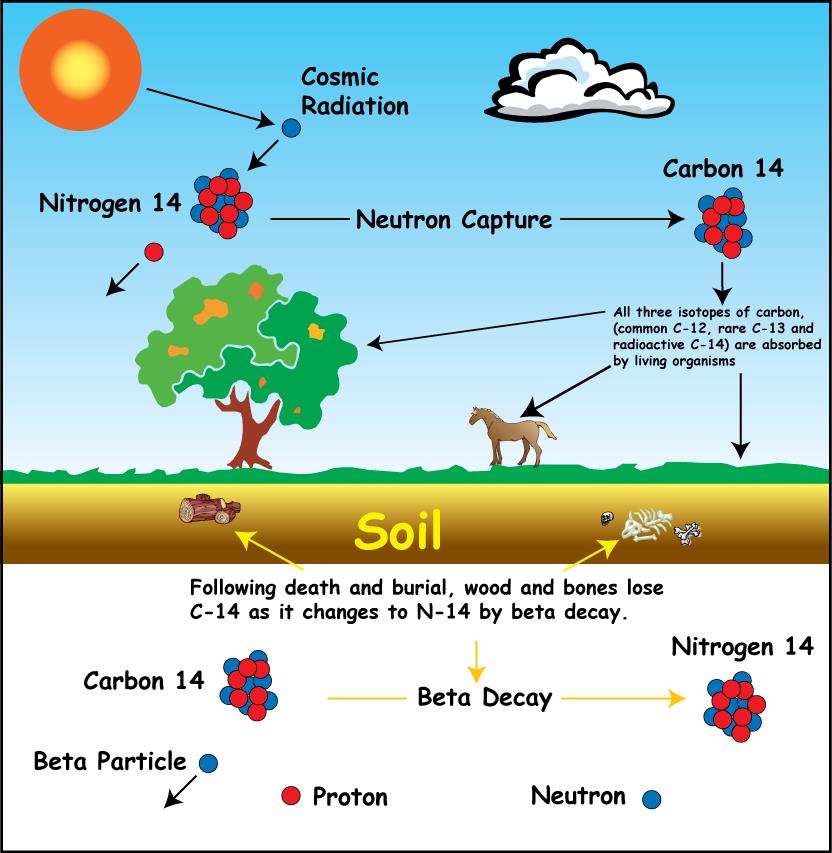
Figure 1. Schematic of 14C production and decay in the atmosphere. 14C is produced in the atmosphere by cosmic neutrons colliding with Nitrogen atoms.  The newly formed 14C is oxidized to 14CO₂ where it then enters the biosphere.  Following an organisms death, radioactive decay occurs converting the 14C back to 14N.

The History of Radiocarbon Dating

Willard Libby invented radiocarbon dating in the late 1940s. His first publication showed the comparisons between known age samples and radiocarbon age (Libby et al, 1949; Libby, 1952). This invention was revolutionary. For the first time it was possible to obtain ages for many events which occurred over the past ~50,000 years. In 1960 Libby was awarded the Nobel Prize for chemistry for this contribution.

Measuring 14C

To obtain the radiocarbon age of a sample it is necessary to determine the proportion of 14C it contains.  Originally this was done by what is known as “conventional” methods, either proportional gas counters or liquid scintillation counters. The gas counter detects the decaying beta particles from a carbon sample that has been converted to a gas (CO₂, methane, acetylene). A liquid scintillation measurement needs the carbon to be converted into benzene, and the instrument then measures the flashes of light (scintillations) as the beta particles interact with a phosphor in the benzene. The main limitation of these techniques is sample size, as hundreds of grams of carbon are needed to count enough decaying beta particles. This is especially true for old samples with low beta activity.  This means that it can be difficult to effectively clean the samples and remove enough contaminating carbon to obtain an accurate date. In the late 1970s and early 1980s the dating of small samples became possible using Accelerator Mass Spectrometry (AMS; Muller, 1977; Nelson et al., 1977). This method needs less than 1 mg of carbon and directly measures the abundance of the individual ions of carbon  (14C, 12C and 13C). 

To obtain a radiocarbon age the sample activity or the 14C/12C ratio must be compared to a standard material of known age. All radiocarbon laboratories either standardize to the US National Bureau of Standards Oxalic Acid I (OX-I) which is derived from Sugar Beets in 1955 or a secondary standard NBS OX-II (grown in 1977) or Australian National University Sucrose (ANU), which is sugar from the 1974 growing season in Australia. Both the OX-II and ANU have been extensively cross-calibrated to OX-I and can be used to normalize a sample for radiocarbon dating. The absolute radiocarbon standard is 1890 wood, the OX-I standard has an activity of 0.95 of this wood.  The definition of year “0”, “modern” or “present” is 1950, there is no real reason for this other than to commemorate the publication of the first radiocarbon dates.

The radiocarbon age is determined by the equation

t = -8033 ln(Asn/Aon)

where -8033 represents the mean lifetime of 14C (Stuiver and Polach, 1977), Asn is the activity in counts per minute of the sample and Aon is the counts per minute of the modern standard. A variant of this equation is also used when the samples are analysed by AMS.  All radiocarbon ages are normalized to a 13C of -25‰ relative to PDB.

Calibration

In the 1950s it was observed that the radiocarbon timescale was not perfect.  The age of known artefacts from Egypt were too young when measured by radiocarbon dating.  A scientist from the Netherlands (Hessel de Vries) tested this by radiocarbon dating tree rings of know ages (de Vries, 1958). He noted some discrepancies indicating that radiocarbon results would need to be “calibrated” to convert them to calendar ages.  de Vries also postulated that the fluctuations were due to the production of 14C and how it changed during variations in cosmic ray production. This brings us to two reasons why a radiocarbon date is not a true calendar age.  The true half-life of 14C is 5730 years and not the originally measured 5568 years used in the radiocarbon age calculation, and the proportion of 14C in the atmosphere is not consistent through time. The latter is due in part to fluctuations in the cosmic ray flux into our atmosphere (e.g. sunspot activity).  Since then there have been many studies examining the variations in the 14C production and its effects on the radiocarbon age to calendar age calibration (e.g. Stuiver, 1971; Edwards et al., 1993; Kitagawa & Van de Plicht, 1998; Stuiver et al., 1998; Fairbanks et al., 2005).  The proportional amount of 14C to total carbon has also changed during the industrial revolution (~1890). Since fossil fuel is derived from millions of year old organic carbon it contains no 14C.  The burning of fossil fuels has caused a dilution of 14C in the atmosphere, this is the so-called “Suess effect” named after Hans Suess (Suess, 1965, 1980). 

It is essential to have radiocarbon ages calibrated to calendar ages so as to have an accurate measure of time. It is also important to be able to compare ages with samples dated by other means, e.g. Uranium Series dating.  It therefore became necessary to create a calibration between radiocarbon dates and calendar age.  The ideal calibration material must have a precise calendar age and sample the atmosphere (carbon reservoir of interest). 

Tree-ring Calibration

Fortunately annual tree rings provide a perfect calibration material available in nature.  Since those first measurements in the 1950s a detailed, precise calibration between radiocarbon and calendar age has been developed using many long-lived tree species. Dendrochronology provides the accurate calendar age for each ring in the tree, and then a radiocarbon age can be assigned to each calendar age. Several tree-ring chronologies have been constructed including the Belfast Irish Oak chronology (Baillie et al. 1983; Brown et al. 1986)  back to ~7200 years and the Stuttgart-Hohenheim oak and pine chronology (e.g. Friedrich et al, 2004; Schaub et al., 2008; Hua et al., 2009) back to ~12, 594 years using thousands of accurately dated tree rings. However this is as far back in time as the continuous tree-ring radiocarbon calibration can be extended at present. More old trees are being discovered every year and this may eventually increase this calibration dataset at a later date.  There are also a number of “floating” tree-ring chronologies that are being developed. They are called floating because they do not have a direct calendar age and must use the radiocarbon to match their ages. For example, many sections of old sub-fossil New Zealand Kauri trees have been found that span time from 25-60,000 years old (Hogg et al., 2006; Turney et al., 2007). 

Calibration Curves

Over the last 20 or so years there have been several calibration “curves” ratified by the Radiocarbon International Community (IntCal98, IntCal04, IntCal09; Stuiver et al., 1998; Reimer et al., 2004, McCormac et al., 2004; Reimer et al., 2009; Reimer et al., 2013; Hogg et al., 2013). Other calibration curves have been proposed by individual research groups (for example Fairbanks et al., 2005), but these have tended to focus on records beyond the Holocene where until very recently there was no consensus on which data should be used. Figure 2 shows the most recent IntCal13 calibration curve superimposed over many of the coral and foram varve  archives.  These calibration curves form the basis of several online calibration programs that take the radiocarbon age and output a calibrated age, the major online calibration programs are;

• Calib – http://intcal.qub.ac.uk/calib/
• CalPal – http://www.calpal.de/
• OxCal – http://c14.arch.ox.ac.uk/embed.php?File=oxcal.html

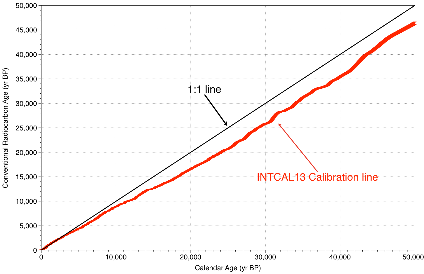
Figure 2. Radiocarbon calibration figure, conventional radiocarbon age on the y-axis vs. Calendar age on the x-axis.  The IntCal13 dataset is used back to 50,000 years BP comprises tree ring data, (Reimer et al., 2013, red line), corals from various locations

Radiocarbon in the Ocean

Marine organisms have a further complication when it comes to radiocarbon dating. The exchange between the ocean and atmospheric 14CO₂ takes on average 10 years to come into equilibrium (Broecker et al., 1985), which never completely happens.  Because the reservoir of carbon in the ocean is so vast and the mixing between the surface and deep ocean is sufficiently long, radioactive decay of carbon in the ocean occurs.  The deep ocean can have an apparent age of several thousand years.  This old carbon mixes upward by a process called “upwelling”. Amounts of upwelling vary throughout the oceans of the world. This results in the surface ocean having an average apparent age of ~400 years, although there is considerable spatial and temporal variability.  This is called the reservoir age or reservoir effect (e.g. Druffel et al., 2008; Eiriksson et al., 2004; Franke et al., 2008). Marine shells of known age collected prior to 1955 and independently dated corals have been used to measure this reservoir variability (e.g. Bourke &Hua, 2009; Culleton et al., 2006; Petchy et al., 2009).  Online databases are available to estimate the reservoir age of a marine sample (Reimer & Reimer, 2009 http://calib.org/marine; Butzin et al., 2005; http://radiocarbon.ldeo.columbia.edu/research/resage.htm).  This is then used to adjust the radiocarbon age and calibrate to a calendar age. A full marine calibration curve is also available (Marine13) to calibrate a marine radiocarbon age, it was calculated using an ocean-atmosphere box diffusion model for the time period 0-10,500 years (Oeschger et al., 1975; Stuiver and Braziunas, 1993) and foram and coral data from 10,500  -12,500 years as describe in Hughen et al. 2004. Beyond 12,500 years the atmospheric calibration curve is used with a constant reservoir age of 405 years (Reimer et al., 2009). 

“Bomb” Radiocarbon

During the 1950s and 1960s nuclear weapons testing generated excess neutrons in the atmosphere thereby creating manmade 14C. This production ceased in 1963 with the signing of the nuclear test ban treaty, however not before the 14C/C ratio in the atmosphere nearly doubled.  This “bomb” radiocarbon has been used to help understand the uptake of CO₂ by the ocean and by the terrestrial biosphere. The subsequent invasion of this “Bomb” 14C into the surface ocean has increased the radiocarbon difference between the surface and the deep ocean (e.g. Broecker, et al., 1985). The use of 14C as a global ocean circulation tracer was a primary objective of the study of the distribution of natural and bomb-produced 14C in the Geochemical Ocean Sections Study (GEOSECS) of the early 1970s (Ostlund and Stuiver, 1980; Broecker et al., 1985) and of the present day World Ocean Circulation Experiment (WOCE; Key et al., 1996).  The GEOSECS data identified a surface water gradient of post-bomb 14C from the equator toward the temperate latitudes.  Broecker and Peng (1982) interpreted this distribution as representing upwelling of low 14C water from the lower thermocline in equatorial regions, with migration of the 14C rich surface water toward higher latitudes.

Radiocarbon measurements of coral skeletal material have been used to study how the radiocarbon content of the tropical surface ocean has varied through time (e.g. Druffel 1981; Guilderson et al., 2000; 2009).  Many coral genera construct massive colonies often 200-400 years old, which in shallow reef environments have growth rates on the order of 1 cm y-1.  Because the radiocarbon in the coral aragonite skeleton reflects seawater radiocarbon content at the time of deposition, radiocarbon measurements across annual skeletal density bands in such corals make it possible to reconstruct the annual mean radiocarbon content of the surface ocean back to pre-bomb and pre-industrial values

Summary

Radiocarbon is a useful means for obtaining the age of death of a carbon-bearing organism.  A robust and internationally agreed calibration has been developed back to 50,000 years ago. Annual tree rings provide the calibration back to ~12,594 yr BP and dated leaves in varved lake deposits alongside speleothems, corals and forams helped refine this calibration back to 50,000 years ago.  Corals have also played a role in trying to understand the oceanic uptake of CO₂ and for tracking ocean currents and circulation.