




NA-Bayes
This page describes the package NA-Bayes. It consists of a set of user callable subroutines which implement the NAB ensemble inference algorithm (the appraisal stage).
The techniques
In June 2005 the code was updated to work in two alternative modes. The original mode whereby all evaluations of the Posterior Probability Density distribution (PPD) are replaced by evaluations of the Neighbourhood approximation of the PPD ; and a new mode, which is a standard MCMC algorithm including actual evaluations of the PPD. With the second mode the code can be used for normal MCMC sampling with all of its graphical output. A summary of changes are described below.Using the Neighbourhood approximation - `NA-bayes' mode
The user specifies a Posterior Probability Density distribution (PPD) and provides an input ensemble of models where the PPD has been evaluated. NAB then uses this ensemble to estimate the values of various Bayesian integrals. No forward modelling is performed. The PPD is approximated everywhere in parameter space using the Neighbourhood approximation of the PPD from the input ensemble (see papers below for a discussion).In principle the input ensemble can follow any distribution and be generated by any search method (e.g. the NA-sampler algorithm, a genetic algorithm or simulated annealing algorithm). A standard Gibbs sampler is then used to provide estimates of Bayesian integrals and their numerical error.
Using full PPD evaluation - `MCMC' mode
The user specifies a Posterior Probability Density distribution (PPD) NAB samples this PPD using a standard Gibbs sampler to estimate values of various Bayesian integrals. Full forward modelling is performed (and code for this is required).Using previously generated samples
For some time the NA-Bayes code has had an option to write out the complete set of parameter space samples generated to a file (nab.samples). See last line of control file nab.in . From May 2006 a feature was added to allow this file to be read back in and used for calculations of marginals. This option is activited by setting the algorithm type to 2 in the second line of nab.in (see below). In this case no new random walks are calculated and no forward modelling performed. The type of weight applied to these samples in the numerical integration depends on their density (e.g. if they were originally created in NA-bayes or MCMC mode in an earlier run). The required information is contained in the header of the file nab.samples and weights are calculated automatically. Note that all information in nab.samples about the original run overrides any conflicting values that may have been set in nab.inThis mode should be very quick. Cases in which you might want to use this are a) if a long run produced a large number of samples and you want to calculate different marginals than the ones in the original run, i.e. by adjusting nab.in (but you don't want to recreate all those samples), or b) the same marginals at a different resolution.
The package
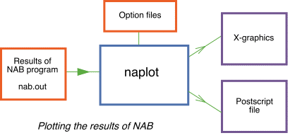
Currently the program produces expectation values of all input variables and any user specified combination of them, 1D and 2D marginals of variables or combinations (including confidence contours), Covariance, Correlation and Resolutions matrices of all variables and combinations. These are out put to a single ascii file nab.out. For convenience a utility plot program called naplot is provided which reads this file and plots the various quantities to an X-window or postscript. (See factors affecting results below.)The package contains source code for the NAB routines and an example driver program. The latter applies the NAB algorithm to the estimation of Bayesian integrals of parameters defining crustal seismic velocity profiles using seismic receiver function data (RFI).
In addition to naplot two other independent utility programs are included. These are fit2ppd which can be used to alter the input ensemble, and combine which can be used to combine the output files of several independent runs of NAB. This makes it possible to run NAB in parallel on multiple machines and simply combine the results at the end. For more information see utility programs. (Note that this program is now redundant since a parallelize version of NAB is included in the distribution (see below ).
This program may be used in conjunction with the author's direct search algorithm NA-sampler. The output of NA-sampler is a direct access `nad file' containing the ensemble of models and their data fits. This same nad file is read in by the NAB program (and fit2ppd).
These pages are meant only as a guide. For more information look at the README files in the src and data directories, the comments in the source code for the RFI example, and the input files for the utility plot programs.- Compiling
- Using the NAB subroutines
- Controlling the Neighbourhood Algorithm
- Factors affecting the accuracy of Bayesian estimators
- Utility programs
- Running the RFI examples
- Conditions of use
- Contacting the author
- Papers and related www sites
Compiling
When the tar file is unpacked it produces four directories:-
src - contains Fortran and C source code for NAB
subroutines and RFI example program and utility/plot programs.
data - contains data input files and example output files
created by RFI example problem.
Also contains the subdirectories naplot and combine
where results can be plotted,
and output files manipulated.
(See utility programs for more details.)
bin - contains executables for RFI example program and all utility programs.
docs - contains these HTML pages.
To compile the complete set of programs
-
> cd src
> make all
If compilation is successful, all executables are placed in the bin directory
and all examples demonstrating the utility programs can be run from the
data directory (See below). The reverse of make all is,
> make clean
which will remove all .o files and all executables.
Note that the Demo directory, the Makefile and the file rfi_nab.f
can serve as a template for new user applications. If you are
not interested in running, or looking at output from the seismic
example program then you can remove all
RFI specific source code and programs with,
> \rm -fr src/utl/fit2ppd/rfi_subs
Note that after this the RFI programs will be gone, the demos
for plot program naplot will not work, and the command
`make all' will no longer work.
A re-installation from a tar file will be necessary to retrieve the
RFI files. It may be best to do this only after you are finished with
the demo examples.
> \rm -fr data/demo_results
> \rm -fr data/fit2ppd/rfi_files
> \rm -fr data/fit2ppd/icov_d50.dat*
Compiling problems
So far I have successfully compiled and run all codes in this package on a SUN workstation (running Solaris 2.7) using both the native compiler and the GNU compilers g77 and gcc, and a DEC alpha (running OSF1 V4.0) using the Digital Fortran and C compilers, and on a Linux machine running SuSEs Linux 7.0 with g77, gcc.
Note that on all platform the direct access files are now written during installation. Disk space savings can be made by deleting the demo files (see above).
If you are using a DEC alpha/compaq platform then you will need to use the compiling option -assume byterecl which makes the Fortran open statement for direct access files the same as on a sun, i.e. with record length specified in bytes rather than words. This can be done by copying the src/makenab.macros_alpha. file to src/makenab.macros.
In the data directory there is an example direct access input file containing an ensemble of seismic velocity models for the RFI problem. It is called `ensemble.nad', which is just a soft link to the file `demo_results/chi_demo.nad'. (NA-Bayes mode only).
Compiling with MPI
To compile using the MPI library and run in a multi-processor environment you need the option -DMPI_NA set as a compiler option. See macros/makenab.macros_intel_mpi for an example. In this case one would normally execute the code using the mpirun (see below).
Code structure and interfacing
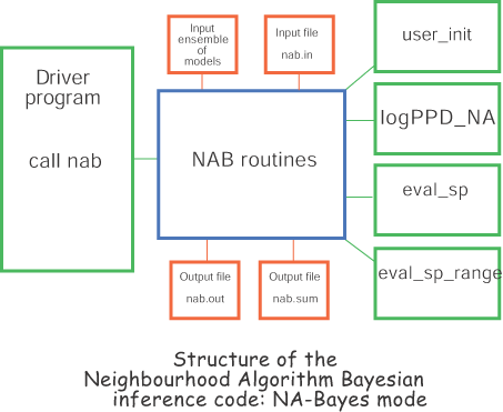
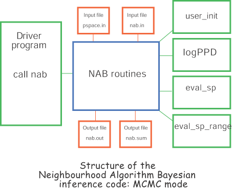
The figure above shows the structure of the NAB code and how it is interfaced with the user code. The green routines must be provided by the user. The main routine passes control to the NAB code by calling the subroutine `nab' with no arguments. This then calls five user written subroutines.
-
user_init - performs any user problem
specific tasks and I/O. Note that the parameter space ranges
and scale factors are read in from the input NAD file.
logPPD - calculates the posterior probability density function at a given input point in parameter space. This routine is only called if MCMC mode is active.
logPPD_NA - calculates the posterior probability density function of the ith member of the input ensemble. (Usually the input ensemble would be pre-processed to contain these values so no forward modelling is required. See utility program fit2ppd below.) Note: this routine was previously called logPPD and is only used if NA-Bayes mode is active.
eval_sp - allows the user to define any number of new variables as function of the original parameter space variables, e.g. if 5 of the normal variables represent thickness of layers within an Earth model, then special variables might be the depth of each interface which are sums of layer thicknesses. All Bayesian measures e.g. standard errors, covariance and expectation etc are calculated for the user defined special variables.
eval_sp_range - defines the upper and lower range of each special variable. (Usually determined from the ranges of the original parameters).
The file rfi_nab.f contains the main driver program and the five subroutines which implement the RFI example problem. In this case the driver routine merely calls nab and exits. The routine user_init is a null routine in the example because no user specific tasks are needed. The five RFI interface routines call no other user specific routines.
To use the NAB subroutines you need to do the following,
- Create the five subroutines for your problem even if some
or most are null routines.
(Use the RFI example as a template) - Create the main routine that calls nab (This can be trivially simple as in the RFI example.)
- Edit the file nab_param.inc to adjust array sizes if necessary.
- Edit the Makefile and makenab.macros to compile the users subroutines
- Compile the new program with
- > make rfi_nab (or the equivalent)
Note that the only essential information that the NAB routines need from the user routines is the definition of the PPD (from logPPD or log_PPD_NA) and any special functions. For NA-Bayes mode the input ensemble, parameter space ranges and scale factors are read in from the input nad file. For more details on the format of the nad file click here. For MCMC mode the parameter space ranges and scale factors are read in from the input file pspace.in.
The development of this code is an ongoing research effort and I expect that the NAB routines will be updated from time to time, however, it is intended that the interface routines will remain unchanged. (The input file nab.in may change.) In this way the incorporation of updated NAB routines into an existing application should be straightforward, i.e. compiling the new nab.f to obtain nab.o and linking with the existing driver code. Note that the NAB source code in sub-directory NAB_src should not normally be edited !
The code was developed on a sun network under Solaris 2.7. Note that there are some issues to consider when transporting the code across to new platforms and compilers systems. The ones that I am aware of are described in the section on Compiling problems. Note that you should specify the platform used by setting the flag in file makenab.macros. You should advise the author if your platform is not supported there.

Controlling the Neighbourhood Bayesian Inference algorithm
The NAB control parameters and other options are read in from the file nab.in.Each line is described below. Note that the control file has changed to accommodate to the two modes of operation.
-
#
# Input options for program NAB
#
0 : forward mode type [0=NA-approximation (NA-Bayes mode), 1=full forward calculation (MCMC mode)]
0 : algorithm type (0=Gibbs sampler, 1=uniform MC integration, 2=read samples from file)
100 : number of random walks used in importance sampling
1000 : number of steps per walk
1 : starting Voronoi cell of first random walk (1=best fit model,2=second best etc)
P : quasi or pseudo-random deviates ? (Q=quasi,P=pseudo)
230728 : random seed (your birthday)
1 : acceptance rate for samples in random walk (thining parameter)
2000 : number of steps before refreshing internal tables (avoids error build up)
y : Turn cpu timing mode on ? (y/n)
100 : Frequency at which diagnostic message is written to standard out
2 : I/O mode (1=silent,2=verbose,3=debug)
20 : Discretization factor for each axis in Gibbs Sampler (only used for MCMC mode)
Options for numerical integration
y
: calculate 1D marginal PDFs ? (y=yes,n=no)
y
: calculate 2D marginal PDFs ? (y=yes,n=no)
y
: calculate covariance matrix ? (y=yes,n=no)
40
: number of bins per axis in 1D marginal pdfs.
20
: number of bins per axis in 2D marginal pdfs.
12
: number of user supplied special functions to integrate (0=none)
22
: number of 2D marginals to calculate (n2d)
32,13
: first pair of variables for 2D marginal (n2d pairs expected)
33,14
: second pair of variables for 2D marginal
.
: ...
.
: ...
.
: ...
100000
: frequency of output to file (in number of samples, -1=Final only)
y
: write out all samples to an ASCI file `nab.samples' (y=yess,n=no)
For NA-bayes mode, the input file format for the ensemble is the same as the output file format for the NA routines, i.e. a direct access nad file which is fully described here. Examples of programs which read and write nad files are contained in the utility programs section.
If a quasi random number generator is not chosen then a pseudo-random number generator is used. (See the papers cited below or Press et al 1992 Numerical Recipes, C.U.P., for a discussion of the difference.)

Output files
nab.sum - Simple summary information of the run.nab.out - All results of Marginals, Covariances and other integrals requested. This file is read by the plot program naplot-x or naplot-p.
nab.samples - Optional out file with all samples used to calculate marginals and integrals. This information can be read back in using input option algorithm type 2 to avoid regeneration of samples. (See above.)
nab.monitor - File containing estimate of how far through the program is at any time. Updated in increments of 5%. Can be useful when a long run (say with full forward modelling is used) and the user wants to know how long it will take to complete.

Factors affecting the accuracy of the Bayesian integrals
There are three factors that affect the overall accuracy of the Bayesian integrals:
The distribution of the input ensemble (NA-bayes mode only)
-
The distribution of the input ensemble of models and their
PPD values define the PPD everywhere in parameter space, and hence
all information available for the Bayesian integrals.
The NAB algorithm assumes nothing about the distribution of the input ensemble.
However, it is self evident that if the input ensemble poorly samples the
PPD then there will be little information to extract from it.
Ideally one should use as big and comprehensive input ensemble
as possible. Usually this would be generated by a direct search algorithm
like the neighbourhood algorithm, or perhaps a genetic algorithm,
or a combination of them.
NAB is then used to estimate Bayesian integrals from this ensemble.
However nothing can make up for a poorly distributed input ensemble.
The form of the posterior probability density distribution
-
In any Bayesian approach the character of the PPD controls the
nature of the problem, and the accuracy of the results.
If the prior information or the likelihood function
are changed in the PPD the obviously the resulting Bayesian
integrals will change.
Here the PPD is defined by the user and it is assumed that this is
appropriate for the problem, noise statistics etc.
The NAB program can do nothing about a poorly or inaccurately
defined PPD.
Convergence of the Gibbs sampler
-
The numerical error in the Bayesian integrals is controlled
by the degree to which the Gibbs samplers (i.e. random walks)
have converged. In principle it is possible to monitor
convergence, estimate numerical error, and adjust the length
and number of walks until the accuracy and convergence estimates
are satisfactory. This of course is at the cost of increased
sampling and hence computation. Since no forward modelling is
performed it is often not too much of a burden to increase
the number and lengths of random walks (see paper below
for more discussion).
In MCMC mode the discretization factor (see input file above) will affect how accurately the PPD is `seen' by the Gibbs sampler. A higher number will be more accurate and a slower running time.
In NAB the estimated numerical error is
calculated for all Bayesian integrals evaluated and can be monitored.
Also the potential scale reduction factor (PSR) is determined for
all expectation values and this indicates how well the random walks
have converged. All values are written out to a table in the
output file nab.out. It looks something like this:
Expectation values
P Mean
Stn err Num err
PSR-stat
1: 1.057292 0.295032 0.053865
1.041
2: 2.262500 0.324244 0.059199
1.064
. .
.
.
.
. .
.
.
.
. .
.
.
.
Convergence is usually assumed satisfactory if all PSR values are less than 1.2 (see paper below for a discussion). If the PSR is greater than this then the number and length of the independent random walks should be increased. Note that in each random walk the Gibbs sampler starts from a different model in the input ensemble. The rank of the model for the first walk is defined in nab.in . Thereafter each walk begins from the next model in descending order. Note also that the importance samples which contribute to the Bayesian integrals are collected from the second half of the walk, i.e. if a walk of length 1000 is specified then a walk of length 2000 steps is performed with the second 1000 models being collected. This dependence on the starting point of the random walk and bias due to `burn in'. (See papers below for more details.)

Utility programs
The following general utility programs are contained in the directory src/utl ,and are run from subdirectories of the data directory.
readnad -

Reads in an ensemble of models in a nad file and writes simple summary information to the screen.
- To read a nad file called `ensemble.nad' then type,
readnad ensemble.nad
fit2ppd -
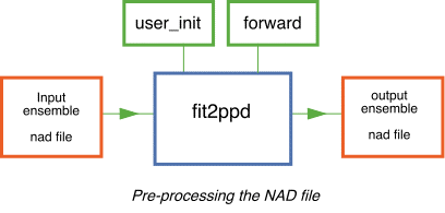
The main purpose of this program is to avoid repetitive forward modelling in the main NAB program. It may also be used to examine the influence of the PPD definition on the results of NAB.
It reads in an input ensemble (nad) file and replaces the misfit function with a new value calculated from calling user supplied forward modelling routines. It then writes out the new nad file which can be input to the main NAB program.
This would normally be used to replace the misfit measure in the nad file with the correct PPD evaluated for each model. This is a pre-processor routine which avoids any forward modelling in the main NAB program. It must be compiled with two user supplied routines `user_init' and `forward' (similar to those in the NA-sampler package). Any other user subroutines that perform forward modelling must also be included.
In the RFI example this program replaces a misfit measure for each model with a Chi-square goodness of fit measure calculated with a non-diagonal data covariance matrix (see paper II below for a discussion). In the main NAB program this chi-square measure is easily converted into a log (PPD) value by the routine logPPD. See the source and Makefile in the directory src/utl/fit2ppd for more details.
- To run fit2ppd type,
fit2ppd ensemble_in.nad ensemble_out.nad
where `ensemble_in.nad' is the original nad file
and `ensemble_out.nad' is the new nad file.
combine -
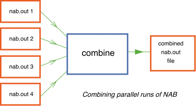
This program is run from the directory data/combine and is used for combining independent output files of NAB run in parallel. For example one might run NAB on ten machines simultaneously each with 100 walks of length 1000, and each starting from different models in the input ensemble, e.g. the first starting at model 1, the second at model 101, the third at 201, etc. By combining the independent runs one can achieve Bayesian integrals evaluated over 1 million samples (with the associated reduction in numerical error) using a tenth of the total cpu time. (This is because the Gibbs sampler's are all independent and hence perfectly parallelizable.) Note that this program is redundant now that an MPI version of the code can be compiled and run.
- To run the combine example type,
combine < comb.in
where `comb.in' contains the number and names of input files.
and output is written to `nab.out'.
naplot -

Running the receiver function inversion example
The example driver program provided with the NA-Bayes package is for the inversion of receiver functions for crustal seismic structure. This is described further in the two NA papers cited below. Note that the driver program is not intended to be a general purpose receiver function code, but merely an example of using the NA routines on a realistic seismic problem. Changes to the code may be required if it is applied to other data sets (For example, the maximum number of layers, and waveforms may need adjusting etc.)
To run the RFI examples after compilation of the package (see above),
-
> cd data
> cp nab.in_test nab.in
> rfi_nab
This will run a short (3 walk) test run with 10 samples generated per walk. This will produce two files nab.sum and nab.out. These should be similar to the file demo_results/nab.sum_test. and demo_results/nab.out_test. A similar set of steps is required to run the longer example in nab.in_full. You could try editing nab.in to adjust input parameters and repeating the test run.
The output file produced by 100 random walks with 1000 samples each is in the demo_results directory. This can be used to demonstrate the features of plot program naplot. See the naplot manual for details of how to run the plot demos.
If the code is compiled with MPI mode then it must be run using your local appropriate MPI command, e.g
-
> cd data
> cp nab.in_test nab.in
> mpirun -np rfi_nab

Format of pspace.in file
When the program is used in MCMC mode. It needs to know what the bounds of the parameter space are, as well as any user defined starting starting points for the Gibbs sampler random walks. (Note in `NA-bayes' mode these are both obtained from the ensemble.nad file). In MCMC mode no nad file is used and so these must be read in from a new file called `pspace.in'. Two examples of pspace.in are provided one for the RFI problem (which contains a 24 parameter problem and 1 special starting point for a random walk) and one for a simple Gaussian (a 12 parameter problem with number of input starting models set to zero). If more random walks are requested in nab.in than there are models in ensemble.nad (NA-Bayes mode) or in pspace.in then random starting points are used. The fortran routine which reads this file is called `read_parameter_space' in src/NAB_src/nab.F and can be consulted if there is any difficulty.

Conditions of use
- 1. The NAB routines may not be distributed to third parties.
Interested parties should contact the author directly.
2. Due acknowledgment must be made of the use of the NA routines in research reports or publications. Whenever such reports are released for public access, a copy should be forwarded to the author.
3. The NAB routines may only be used for research and development, unless it has been agreed otherwise with the author in writing.

Contacting the author
The purpose of this documentation and the associated README files, is to reduce the likelihood of running into problems. I would be grateful if you do not contact me with queries on the installation, or running, of the code unless you have thoroughly looked for the answer yourself. (Note that either these pages, the README files, example files and the source code itself may provide an answer).
I am very interested in obtaining feedback on people's experiences with
this code. Especially to hear what type of problems it has been applied
to.
I expect that the code will be updated from time to time.
Information on new developments will be posted on the
NA homepage.

Related links:
- NA homepage - where the latest versions of NA-Bayes and NA-sampler can be accessed.
- NA-sampler - the manual for the neighbourhood algorithm direct search package.
- NA-Bayes - the latest version of this manual.
- naplot - graphics program for displaying Bayesian estimators.
- splot - graphics program for display of multi-dimensional ensembles.
- NAD - explanation of direct access nad files.
- RFI - Receiver function utility programs and graphics.
- Malcolm's homepage

References:
-
The Neighbourhood algorithm for searching a multi-dimensional parameter space
for models (points) with `acceptable data fit' is implemented
in the author's program NA-Sampler, and is described in the paper:
Geophysical Inversion with a Neighbourhood Algorithm I: searching
a parameter space,
Sambridge, M., Geophys. J. Int., 138,
479-494, 1999.
The algorithm in package NA-Bayes for calculating Bayesian integrals from a finite ensemble is presented in the paper:
Geophysical Inversion with a Neighbourhood Algorithm II: appraising
the ensemble,
Sambridge, M., Geophys. J. Int., 138,
727-746, 1999.
Postscript and PDF files of these papers can be downloaded from the NA homepage. Also related sites and references on this work can be found there.

Enquires to Malcolm Sambridge: malcolm@rses.anu.edu.au

Last modified May 2006.